
Sensitivity Analysis#
An overall success rate tells you how often a policy completed the task, but not which tested conditions were associated with success. Sensitivity analysis connects each episode’s outcome to the conditions sampled during that episode.
Sensitivity analysis can help you:
Find a robust operating range. See whether success is associated with a broad part of the tested range or only a narrow region.
Identify the most sensitive factors. Compare the posteriors to see which conditions constrain the policy most strongly.
Target additional training data. Collect or augment data across sensitive conditions to improve the policy’s robustness.
Compare policies. Repeat the same sweep for multiple policies and compare their sensitivity alongside their overall success rates.
This workflow continues from Run an Evaluation. It uses the saved episode results to estimate the posterior distribution over wrist-camera offsets conditioned on success. Arena models the selected factors together, then displays one marginal posterior for each camera axis. This is not a success-rate-versus-offset plot.
The earlier sweep is deliberately small: it demonstrates the workflow, but it is not enough to judge the policy’s robustness. For background on the method, see the Sensitivity Analysis concept page.
Estimate the success-conditioned posterior#
In the Base Docker container, set the paths used by the download and analysis commands:
export CAMERA_SENSITIVITY_OUTPUT_DIR="/eval/camera_sensitivity_workflow"
RUN_OUTPUT_DIRECTORY="${CAMERA_SENSITIVITY_OUTPUT_DIR}/droid_pnp_camera_sensitivity_openpi"
EPISODE_RESULTS_PATH="${RUN_OUTPUT_DIRECTORY}/episode_results_rebuild0.jsonl"
POSTERIOR_FIGURE_PATH="${RUN_OUTPUT_DIRECTORY}/camera_sensitivity_posterior.png"
To start here without running the evaluation workflow, download the saved episode results:
Download episode results (skip evaluation workflow)
These commands download a small sample of episode results from the camera-sensitivity experiment, so you can follow this workflow without first running the variation sweep.
mkdir -p "${RUN_OUTPUT_DIRECTORY}"

HF_DATASET_REPOSITORY="nvidia/Arena-DROID-Camera-Sensitivity-Workflow-Sample"
HF_DATASET_REVISION="arena_v0.2_lab_v3.0"

hf download \
  "${HF_DATASET_REPOSITORY}" \
  episode_results_rebuild0.jsonl \
  --repo-type dataset \
  --revision "${HF_DATASET_REVISION}" \
  --local-dir "${RUN_OUTPUT_DIRECTORY}"
Whether generated by the evaluation workflow or downloaded above, the results are stored in
${RUN_OUTPUT_DIRECTORY}. Run:
python -m isaaclab_arena.analysis.sensitivity.generate_report \
  --episode_results "${EPISODE_RESULTS_PATH}" \
  --outcome success \
  --factors droid_abs_joint_pos.camera_extrinsics_wrist_camera \
  --output "${POSTERIOR_FIGURE_PATH}"
This command trains a neural posterior estimator (NPE) on all episodes in the JSONL file and
writes the resulting posterior-marginal plot to ${POSTERIOR_FIGURE_PATH}, which we inspect in
the next step.
For the downloaded sample, the terminal output includes:
[INFO] SensitivityAnalyzer: fitting NPE_C on 10 episodes (theta dim=3, x dim=1).
...
[INFO] Wrote report → /eval/camera_sensitivity_workflow/droid_pnp_camera_sensitivity_openpi/camera_sensitivity_posterior.png
Read the posterior marginals#
Still in the Base Docker container, open the generated image:
NO_AT_BRIDGE=1 pqiv "${POSTERIOR_FIGURE_PATH}"
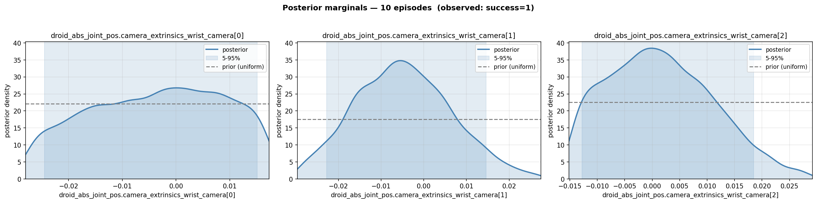
Posterior marginals generated from the small camera-position sweep in the evaluation workflow.#
Each panel shows the marginal posterior for one component of the wrist-camera offset, measured in metres. In the camera’s optical frame:
[0]is horizontal displacement: negative moves left and positive moves right;[1]is vertical displacement: negative moves up and positive moves down; and[2]is depth displacement: negative moves backward and positive moves forward.
The blue curve is the estimated posterior density conditioned on success. The grey dashed line is a uniform reference over the recorded range. A curve close to the dashed line suggests no clear association in the recorded data. A curve concentrated in part of the range suggests that those values are more strongly associated with successful episodes.
Turn the posterior into practical takeaways#
Because this walkthrough uses a small sweep, the interpretation below is hypothetical. If the same posterior shapes persisted in a larger experiment, they would support these takeaways:
Horizontal offset ([0]): The broad posterior suggests less sensitivity to left-right camera offsets than to the other axes.
Vertical offset ([1]): The narrow posterior peaks at a small upward offset. Check the camera calibration and mounting position before deployment.
Depth offset ([2]): The posterior peaks near nominal and declines for forward offsets. Keep the camera standoff close to nominal and limit forward mounting error.
Together, these results make vertical and depth alignment the priorities for camera mounting, calibration, and additional training data. Horizontal alignment can allow more variation over the tested range.
Finally, each panel is a marginal of the joint posterior. The three individual peaks do not necessarily form the best combined camera position: one offset may compensate for another. Use a joint or pairwise posterior view before choosing a new three-dimensional mounting transform.
Scale up with a multi-node evaluation#
The local sweep demonstrates how recorded episodes become posterior marginals. Sensitivity analysis typically needs many rollouts for a reliable estimate. Continue to Multi-Node Evaluation to distribute a larger sweep across a cluster and analyze its collected results.