Training a Gear Insertion Policy and ROS Deployment

Training a Gear Insertion Policy and ROS Deployment#

This tutorial walks you through how to train a gear insertion assembly reinforcement learning (RL) policy that transfers from simulation to a real robot. The workflow consists of two main stages:

Simulation Training in Isaac Lab: Train the policy in a high-fidelity physics simulation with domain randomization
Real Robot Deployment with Isaac ROS: Deploy the trained policy on real hardware using Isaac ROS and a custom ROS inference node

This walkthrough covers the key principles and best practices for sim-to-real transfer using Isaac Lab, illustrated with a real-world example:

the Gear Assembly task for the UR10e robot with the Robotiq 2F-140 gripper or 2F-85 gripper

Task Details:

The gear assembly policy operates as follows:

Initial State: The policy assumes the gear is already grasped by the gripper at the start of the episode
Input Observations: The policy receives the pose of the gear shaft (position and orientation) in which the gear should be inserted, obtained from a separate perception pipeline
Policy Output: The policy outputs delta joint positions (incremental changes to joint angles) to control the robot arm and perform the insertion
Generalization: The trained policy generalizes across 3 different gear sizes without requiring retraining for each size

Sim-to-real transfer: Gear assembly policy trained in Isaac Lab (left) successfully deployed on real UR10e robot (right).#

This environment has been successfully deployed on real UR10e robots without an IsaacLab dependency.

Scope of This Tutorial:

This tutorial focuses exclusively on the training part of the sim-to-real transfer workflow in Isaac Lab. For the complete deployment workflow on the real robot, including the exact steps to set up the vision pipeline, robot interface and the ROS inference node to run your trained policy on real hardware, please refer to the Isaac ROS Documentation.

Overview#

Successful sim-to-real transfer requires addressing three fundamental aspects:

Input Consistency: Ensuring the observations your policy receives in simulation match those available on the real robot
System Response Consistency: Ensuring the robot and environment respond to actions in simulation the same way they do in reality
Output Consistency: Ensuring any post-processing applied to policy outputs in Isaac Lab is also applied during real-world inference

When all three aspects are properly addressed, policies trained purely in simulation can achieve robust performance on real hardware without any real-world training data.

Debugging Tip: When your policy fails on the real robot, the best approach to debug is to set up the real robot with the same initial observations as in simulation, then compare how the controller/system respond. This isolates whether the problem is from observation mismatch (Input Consistency) or physics/controller mismatch (System Response Consistency).

Part 1: Input Consistency#

The observations your policy receives must be consistent between simulation and reality. This means:

The observation space should only include information available from real sensors
Sensor noise and delays should be modeled appropriately

Using Real-Robot-Available Observations#

Your simulation environment should only use observations that are available on the real robot and not use “privileged” information that wouldn’t be available in deployment.

Observation Specification: Isaac-Deploy-GearAssembly-UR10e-2F140-v0#

The Gear Assembly environment uses both proprioceptive and exteroceptive (vision) observations:

Gear Assembly Environment Observations#
Observation	Dimension	Real-World Source	Noise in Training
`joint_pos`	6 (UR10e arm joints)	UR10e controller	None (proprioceptive)
`joint_vel`	6 (UR10e arm joints)	UR10e controller	None (proprioceptive)
`gear_shaft_pos`	3 (x, y, z position)	FoundationPose + RealSense depth	±0.005 m (5mm, estimated error from FoundationPose + RealSense depth pipeline)
`gear_shaft_quat`	4 (quaternion orientation)	FoundationPose + RealSense depth	±0.01 per component (~5° angular error, estimated error from FoundationPose + RealSense depth pipeline)

Implementation:

from isaaclab.utils.noise import AdditiveUniformNoiseCfg as Unoise

@configclass
class PolicyCfg(ObsGroup):
    """Observations for policy group."""

    # Robot joint states - NO noise for proprioceptive observations
    joint_pos = ObsTerm(
        func=mdp.joint_pos,
        params={"asset_cfg": SceneEntityCfg("robot", joint_names=["shoulder_pan_joint", ...])},
    )

    joint_vel = ObsTerm(
        func=mdp.joint_vel,
        params={"asset_cfg": SceneEntityCfg("robot", joint_names=["shoulder_pan_joint", ...])},
    )

    # Gear shaft pose from FoundationPose perception
    # ADD noise for exteroceptive (vision-based) observations
    # Calibrated to match FoundationPose + RealSense D435 error
    # Typical error: 3-8mm position, 3-7° orientation
    gear_shaft_pos = ObsTerm(
        func=mdp.gear_shaft_pos_w,
        params={"asset_cfg": SceneEntityCfg("factory_gear_base")},
        noise=Unoise(n_min=-0.005, n_max=0.005),  # ±5mm
    )

    # Quaternion noise: small uniform noise on each component
    # Results in ~5° orientation error
    gear_shaft_quat = ObsTerm(
        func=mdp.gear_shaft_quat_w,
        params={"asset_cfg": SceneEntityCfg("factory_gear_base")},
        noise=Unoise(n_min=-0.01, n_max=0.01),
    )

    def __post_init__(self):
        self.enable_corruption = True  # Enable for perception observations only
        self.concatenate_terms = True

Why No Noise for Proprioceptive Observations?

Empirically, we found that policies trained without noise on proprioceptive observations (joint positions and velocities) transfer well to real hardware. The UR10e controller provides sufficiently accurate joint state feedback that modeling sensor noise doesn’t improve sim-to-real transfer for these tasks.

Part 2: System Response Consistency#

Once your observations are consistent, you need to ensure the simulated robot and environment respond to actions the same way the real system does. In this use case, this involves three main aspects:

Physics simulation parameters (friction, contact properties)
Actuator modeling (PD controller gains, effort limits)
Domain randomization

Physics Parameter Tuning#

Accurate physics simulation is critical for contact-rich tasks. Key parameters include:

Friction coefficients (static and dynamic)
Contact solver parameters
Material properties
Rigid body properties

Example: Gear Assembly Physics Configuration

The Gear Assembly task requires accurate contact modeling for insertion. Here’s how friction is configured:

# From joint_pos_env_cfg.py in Isaac-Deploy-GearAssembly-UR10e-2F140-v0

@configclass
class EventCfg:
    """Configuration for events including physics randomization."""

    # Randomize friction for gear objects
    small_gear_physics_material = EventTerm(
        func=mdp.randomize_rigid_body_material,
        mode="startup",
        params={
            "asset_cfg": SceneEntityCfg("factory_gear_small", body_names=".*"),
            "static_friction_range": (0.75, 0.75),   # Calibrated to real gear material
            "dynamic_friction_range": (0.75, 0.75),
            "restitution_range": (0.0, 0.0),         # No bounce
            "num_buckets": 16,
        },
    )

    # Similar configuration for gripper fingers
    robot_physics_material = EventTerm(
        func=mdp.randomize_rigid_body_material,
        mode="startup",
        params={
            "asset_cfg": SceneEntityCfg("robot", body_names=".*finger"),
            "static_friction_range": (0.75, 0.75),   # Calibrated to real gripper
            "dynamic_friction_range": (0.75, 0.75),
            "restitution_range": (0.0, 0.0),
            "num_buckets": 16,
        },
    )

These friction values (0.75) were determined through iterative visual comparison:

Record videos of the gear being grasped and manipulated on real hardware
Start training in simulation and observe the live simulation viewer
Look for physics issues (penetration, unrealistic slipping, poor contact)
Adjust friction coefficients and solver parameters and retry
Compare the gear’s behavior in the gripper visually between sim and real
Repeat adjustments until behavior matches (no need to wait for full policy training)

Once physics looks good, train in headless mode with video recording:

python scripts/reinforcement_learning/rsl_rl/train.py \
    --task Isaac-Deploy-GearAssembly-UR10e-2F140-v0 \
    --headless \
    --video --video_length 800 --video_interval 5000

Review the recorded videos and compare with real hardware videos to verify physics behavior

Contact Solver Configuration

Contact-rich manipulation requires careful solver tuning. These parameters were calibrated through the same iterative visual comparison process as the friction coefficients:

# Robot rigid body properties
rigid_props=sim_utils.RigidBodyPropertiesCfg(
    disable_gravity=True,                    # Robot is mounted, no gravity
    max_depenetration_velocity=5.0,          # Control interpenetration resolution
    linear_damping=0.0,                      # No artificial damping
    angular_damping=0.0,
    max_linear_velocity=1000.0,
    max_angular_velocity=3666.0,
    enable_gyroscopic_forces=True,           # Important for accurate dynamics
    solver_position_iteration_count=4,       # Balance accuracy vs performance
    solver_velocity_iteration_count=1,
    max_contact_impulse=1e32,               # Allow large contact forces
),

Important: The solver_position_iteration_count is a critical parameter for contact-rich tasks. Increasing this value improves collision simulation stability and reduces penetration issues, but it also increases simulation and training time. For the gear assembly task, we use solver_position_iteration_count=4 as a balance between physics accuracy and computational performance. If you observe penetration or unstable contacts, try increasing to 8 or 16, but expect slower training.

# Articulation properties
articulation_props=sim_utils.ArticulationRootPropertiesCfg(
    enabled_self_collisions=False,
    solver_position_iteration_count=4,
    solver_velocity_iteration_count=1,
),

# Contact properties
collision_props=sim_utils.CollisionPropertiesCfg(
    contact_offset=0.005,                    # 5mm contact detection distance
    rest_offset=0.0,                         # Objects touch at 0 distance
),

Actuator Modeling#

Accurate actuator modeling ensures the simulated robot moves like the real one. This includes:

PD controller gains (stiffness and damping)
Effort and velocity limits
Joint friction

Controller Choice: Impedance Control

For the UR10e deployment, we use an impedance controller interface. Using a simpler controller like impedance control reduces the chances of variation between simulation and reality compared to more complex controllers (e.g., operational space control, hybrid force-position control). Simpler controllers:

Have fewer parameters that can mismatch between sim and real
Are easier to model accurately in simulation
Have more predictable behavior that’s easier to replicate
Reduce the controller complexity as a source of sim-real gap

Example: UR10e Actuator Configuration

# Default UR10e actuator configuration
actuators = {
    "arm": ImplicitActuatorCfg(
        joint_names_expr=["shoulder_pan_joint", "shoulder_lift_joint",
                        "elbow_joint", "wrist_1_joint", "wrist_2_joint", "wrist_3_joint"],
        effort_limit=87.0,           # From UR10e specifications
        velocity_limit=2.0,          # From UR10e specifications
        stiffness=800.0,             # Calibrated to match real behavior
        damping=40.0,                # Calibrated to match real behavior
    ),
}

Domain Randomization of Actuator Parameters

To account for variations in real robot behavior, randomize actuator gains during training:

# From EventCfg in the Gear Assembly environment
robot_joint_stiffness_and_damping = EventTerm(
    func=mdp.randomize_actuator_gains,
    mode="reset",
    params={
        "asset_cfg": SceneEntityCfg("robot", joint_names=["shoulder_.*", "elbow_.*", "wrist_.*"]),
        "stiffness_distribution_params": (0.75, 1.5),    # 75% to 150% of nominal
        "damping_distribution_params": (0.3, 3.0),       # 30% to 300% of nominal
        "operation": "scale",
        "distribution": "log_uniform",
    },
)

Joint Friction Randomization

Real robots have friction in their joints that varies with position, velocity, and temperature. For the UR10e with impedance controller interface, we observed significant stiction (static friction) causing the controller to not reach target joint positions.

Characterizing Real Robot Behavior:

To quantify this behavior, we plotted the step response of the impedance controller on the real robot and observed contact offsets of approximately 0.25 degrees from the commanded setpoint. This steady-state error is caused by joint friction opposing the controller’s commanded motion. Based on these measurements, we added joint friction modeling in simulation to replicate this behavior:

joint_friction = EventTerm(
    func=mdp.randomize_joint_parameters,
    mode="reset",
    params={
        "asset_cfg": SceneEntityCfg("robot", joint_names=["shoulder_.*", "elbow_.*", "wrist_.*"]),
        "friction_distribution_params": (0.3, 0.7),     # Add 0.3 to 0.7 Nm friction
        "operation": "add",
        "distribution": "uniform",
    },
)

Why Joint Friction Matters: Without modeling joint friction in simulation, the policy learns to expect that commanded joint positions are always reached. On the real robot, stiction prevents small movements and causes steady-state errors. By adding friction during training, the policy learns to account for these effects and commands appropriately larger motions to overcome friction.

Compensating for Stiction with Action Scaling:

To help the policy overcome stiction on the real robot, we also increased the output action scaling. The Isaac ROS documentation notes that a higher action scale (0.0325 vs 0.025) is needed to overcome the higher static friction (stiction) compared to the 2F-85 gripper. This increased scaling ensures the policy commands are large enough to overcome the friction forces observed in the step response analysis.

Action Space Design#

Your action space should match what the real robot controller can execute. For this task we found that incremental joint position control is the most reliable approach.

Example: Gear Assembly Action Configuration

# For contact-rich manipulation, smaller action scale for more precise control
self.joint_action_scale = 0.025  # ±2.5 degrees per step

self.actions.arm_action = mdp.RelativeJointPositionActionCfg(
    asset_name="robot",
    joint_names=["shoulder_pan_joint", "shoulder_lift_joint", "elbow_joint",
                "wrist_1_joint", "wrist_2_joint", "wrist_3_joint"],
    scale=self.joint_action_scale,
    use_zero_offset=True,
)

The action scale is a critical hyperparameter that should be tuned based on:

Task precision requirements (smaller for contact-rich tasks)
Control frequency (higher frequency allows larger steps)

Domain Randomization Strategy#

Domain randomization should cover the range of conditions in which you want the real robot to perform. Increasing randomization ranges makes it harder for the policy to learn, but allows for larger variations in inputs and system parameters. The key is to balance training difficulty with robustness: randomize enough to cover real-world variations, but not so much that the policy cannot learn effectively.

Pose Randomization

For manipulation tasks, randomize object poses to ensure the policy works across the workspace:

# From Gear Assembly environment
randomize_gears_and_base_pose = EventTerm(
    func=gear_assembly_events.randomize_gears_and_base_pose,
    mode="reset",
    params={
        "pose_range": {
            "x": [-0.1, 0.1],                          # ±10cm
            "y": [-0.25, 0.25],                        # ±25cm
            "z": [-0.1, 0.1],                          # ±10cm
            "roll": [-math.pi/90, math.pi/90],         # ±2 degrees
            "pitch": [-math.pi/90, math.pi/90],        # ±2 degrees
            "yaw": [-math.pi/6, math.pi/6],            # ±30 degrees
        },
        "gear_pos_range": {
            "x": [-0.02, 0.02],                        # ±2cm relative to base
            "y": [-0.02, 0.02],
            "z": [0.0575, 0.0775],                     # 5.75-7.75cm above base
        },
        "rot_randomization_range": {
            "roll": [-math.pi/36, math.pi/36],         # ±5 degrees
            "pitch": [-math.pi/36, math.pi/36],
            "yaw": [-math.pi/36, math.pi/36],
        },
    },
)

Initial State Randomization

Randomizing the robot’s initial configuration helps the policy handle different starting conditions:

set_robot_to_grasp_pose = EventTerm(
    func=gear_assembly_events.set_robot_to_grasp_pose,
    mode="reset",
    params={
        "robot_asset_cfg": SceneEntityCfg("robot"),
        "rot_offset": [0.0, math.sqrt(2)/2, math.sqrt(2)/2, 0.0],  # Base gripper orientation
        "pos_randomization_range": {
            "x": [-0.0, 0.0],
            "y": [-0.005, 0.005],                      # ±5mm variation
            "z": [-0.003, 0.003],                      # ±3mm variation
        },
        "gripper_type": "2f_140",
    },
)

Part 3: Training the Policy in Isaac Lab#

Now that we’ve covered the key principles for sim-to-real transfer, let’s train the gear assembly policy in Isaac Lab.

Step 1: Visualize the Environment#

First, launch the training with a small number of environments and visualization enabled to verify that the environment is set up correctly:

# Launch training with visualization
python scripts/reinforcement_learning/rsl_rl/train.py \
    --task Isaac-Deploy-GearAssembly-UR10e-2F140-v0 \
    --num_envs 4

Note

For the Robotiq 2F-85 gripper, use --task Isaac-Deploy-GearAssembly-UR10e-2F85-v0 instead.

This will open the Isaac Sim viewer where you can observe the training process in real-time.

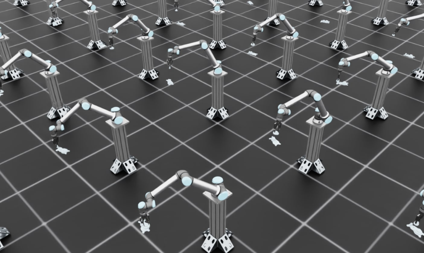
Gear assembly training visualization in Isaac Lab — Training visualization showing multiple parallel environments with robots grasping gears.#

What to Expect:

In the early stages of training, you should see the robots moving around with the gears grasped by the grippers, but they won’t be successfully inserting the gears yet. This is expected behavior as the policy is still learning. The robots will move the grasped gear in various directions. Once you’ve verified the environment looks correct, stop the training (Ctrl+C) and proceed to full-scale training.

Step 2: Full-Scale Training with Video Recording#

Now launch the full training run with more parallel environments in headless mode for faster training. We’ll also enable video recording to monitor progress:

# Full training with video recording
python scripts/reinforcement_learning/rsl_rl/train.py \
    --task Isaac-Deploy-GearAssembly-UR10e-2F140-v0 \
    --headless \
    --num_envs 256 \
    --video --video_length 800 --video_interval 5000

This command will:

Run 256 parallel environments for efficient training
Run in headless mode (no visualization) for maximum performance
Record videos every 5000 steps to monitor training progress
Save videos with 800 frames each

Training typically takes ~12-24 hours for a robust insertion policy. The videos will be saved in the logs directory and can be reviewed to assess policy performance during training.

Note

GPU Memory Considerations: The default configuration uses 256 parallel environments, which should work on most modern GPUs (e.g., RTX 3090, RTX 4090, A100). For better sim-to-real transfer performance, you can increase solver_position_iteration_count from 4 to 196 in gear_assembly_env_cfg.py and joint_pos_env_cfg.py for more realistic contact simulation, but this requires a larger GPU (e.g., RTX PRO 6000 with 40GB+ VRAM). Higher solver iteration counts reduce penetration and improve contact stability but significantly increase GPU memory usage.

Monitoring Training Progress with TensorBoard:

You can monitor training metrics in real-time using TensorBoard. Open a new terminal and run:

./isaaclab.sh -p -m tensorboard.main --logdir <log_dir>

Replace <log_dir> with the path to your training logs (e.g., logs/rsl_rl/gear_assembly_ur10e/2025-11-19_19-31-01). TensorBoard will display plots showing rewards, episode lengths, and other metrics. Verify that the rewards are increasing over iterations to ensure the policy is learning successfully.

Step 3: Deploy on Real Robot#

Once training is complete, follow the Isaac ROS inference documentation to deploy your policy.

The Isaac ROS deployment pipeline directly uses the trained model checkpoint (.pt file) along with the agent.yaml and env.yaml configuration files generated during training. No additional export step is required.

The deployment pipeline uses Isaac ROS and a custom ROS inference node to run the policy on real hardware. The pipeline includes:

Perception: Camera-based pose estimation (FoundationPose, Segment Anything)
Motion Planning: cuMotion for collision-free trajectories
Policy Inference: Your trained policy running at control frequency in a custom ROS inference node
Robot Control: Low-level controller executing commands

Troubleshooting#

This section covers common errors you may encounter during training and their solutions.

PhysX Collision Stack Overflow#

Error Message:

PhysX error: PxGpuDynamicsMemoryConfig::collisionStackSize buffer overflow detected,
please increase its size to at least 269452544 in the scene desc!
Contacts have been dropped.

Cause: This error occurs when the GPU collision detection buffer is too small for the number of contacts being simulated. This is common in contact-rich environments like gear assembly.

Solution: Increase the gpu_collision_stack_size parameter in gear_assembly_env_cfg.py:

# In GearAssemblyEnvCfg class
sim: SimulationCfg = SimulationCfg(
    physx=PhysxCfg(
        gpu_collision_stack_size=2**31,  # Increase this value if you see overflow errors
        gpu_max_rigid_contact_count=2**23,
        gpu_max_rigid_patch_count=2**23,
    ),
)

The error message will suggest a minimum size. Set gpu_collision_stack_size to at least the recommended value (e.g., if the error says “at least 269452544”, set it to 2**28 or 2**29). Note that increasing this value increases GPU memory usage.

CUDA Out of Memory#